Mathematical Foundations and Correctness Testing

Overview

This document describes the mathematical foundations of the 3D finite-difference stencil computation, the methods used to identify and characterize the underlying partial differential equation, and how these foundations inform our definition of correctness and testing methodology.

Equation Identification

Underlying PDE: 3D Wave Equation

The reference implementation solves the 3D wave equation:

\[\frac{\partial^2 u}{\partial t^2} = c^2 \nabla^2 u + f(x,y,z,t)\]

Where:

• $u(x,y,z,t)$ is the wave field
• $c$ is the wave speed (encoded in material parameter $m$)
• $f$ is the source term
• $\nabla^2$ is the 3D Laplacian operator

Numerical Scheme

Spatial Discretization: 4th-order finite difference

• Stencil: 5-point centered difference in each dimension
• Accuracy: O(h⁴) in space
• Formula: \(\frac{\partial^2 u}{\partial x^2} \approx \frac{-u_{i-2} + 16u_{i-1} - 30u_i + 16u_{i+1} - u_{i+2}}{12h^2}\)

Temporal Discretization: 2nd-order finite difference

• Accuracy: O(Δt²) in time
• Leapfrog structure: Uses three time levels (t0, t1, t2)

Evidence from Code Analysis

The update equation in ref/code.cpp implements:

u[t2] = dt² * (spatial_terms - temporal_terms) / m

Where:

• Spatial terms: 4th-order finite difference Laplacian in x, y, z
• Temporal terms: r1 * (u[t1] - 2*u[t0]) providing the leapfrog structure
• Material properties: m affects wave speed and energy conservation

Stability Analysis

Von Neumann Stability Method

Von Neumann stability analysis determines whether a finite difference scheme remains bounded over time by:

1. Fourier Decomposition: Express the solution as a sum of Fourier modes
2. Amplification Factor: Determine how each mode evolves: $u^{n+1} = G(k) u^n$

3. Stability Criterion: Ensure $

   G(k)

   \leq 1$ for all wavenumbers $k$

Stability Results

Critical CFL Number: 0.5 (empirically determined)

• Stable Range: CFL < 0.5
• Unstable Range: CFL ≥ 0.5 (produces NaN/Inf)
• Theoretical Limit: CFL ≤ 0.5 for 4th-order finite difference schemes in 3D

Key Finding: The scheme follows standard 4th-order finite difference stability limits, consistent with theoretical expectations for the 3D wave equation.

Implications for Testing

1. CFL Constraint: All correctness tests must use CFL < 0.5
2. Stability Validation: Long-time integration tests verify boundedness
3. Parameter Space: Testing must cover stable and near-unstable regimes

Accuracy Analysis

Modified Wavenumber Analysis

The finite difference scheme introduces numerical dispersion:

• Phase Velocity Error: Up to 26.5% at highest wavenumbers
• Resolution Requirements:
  • 1% error: 5.27 points per wavelength
  • 5% error: 3.39 points per wavelength
  • 10% error: 2.76 points per wavelength

Discretization Order Verification

Empirical convergence analysis confirms:

• Spatial order: 4th-order (O(h⁴)) convergence
• Temporal order: 2nd-order (O(Δt²)) convergence

This is verified through:

• Grid refinement studies
• Comparison with analytical solutions
• Error norm analysis (L2, L∞)

Defining Correctness

Levels of Correctness

1. Numerical Parity: CUDA kernel produces identical results to CPU reference
   • Tolerance: Checksum difference < 1e-5
   • Method: Per-voxel comparison after identical timesteps
   • Rationale: Same mathematical scheme should produce same results
2. Physical Correctness: Solution satisfies wave equation properties
   • Energy Conservation: Total energy remains bounded (for closed systems)
   • Wave Propagation: Solutions propagate at correct speed
   • Boundary Behavior: Appropriate boundary condition handling
3. Stability: Solution remains bounded for stable CFL numbers
   • Long-time Integration: No exponential growth for CFL < 0.5
   • Error Accumulation: Errors grow at expected rate (not catastrophically)
4. Convergence: Solution converges to analytical solution as grid refines
   • Spatial Convergence: 4th-order rate
   • Temporal Convergence: 2nd-order rate

Correctness Testing Methodology

1. Parity Testing

Purpose: Verify CUDA kernel implements the same numerical scheme as CPU reference.

Method:

• Initialize identical initial conditions
• Run same number of timesteps with identical parameters
• Compare final state (checksum, max difference, L2 norm)

Criteria:

• Checksum difference < 1e-5
• Max per-voxel difference < 1e-5
• L2 norm difference < 1e-5

Rationale: If the numerical scheme is identical, floating-point differences should be minimal (within roundoff).

2. Analytical Solution Validation

Purpose: Verify the scheme solves the correct PDE with expected accuracy.

Method:

• Use known analytical solutions (Gaussian pulse, plane wave, standing wave)
• Compare numerical solution to analytical solution
• Measure convergence rate with grid refinement

Criteria:

• L2 error decreases with expected order (4th-order spatial, 2nd-order temporal)
• Error magnitude consistent with discretization order

Rationale: Correct PDE + correct scheme → correct solution (up to discretization error).

3. Stability Testing

Purpose: Verify the scheme remains stable for appropriate parameter ranges.

Method:

• Run long-time integrations (many timesteps)
• Test various CFL numbers (0.1, 0.2, 0.3, 0.4, 0.5)
• Monitor solution growth/decay

Criteria:

• Solution remains bounded for CFL < 0.5
• No NaN/Inf for stable CFL numbers
• Energy conservation (for appropriate boundary conditions)

Rationale: Unstable schemes produce unphysical results, violating correctness.

4. Order Verification

Purpose: Confirm the scheme achieves expected discretization order.

Method:

• Grid refinement study (h → h/2 → h/4)
• Measure error vs grid spacing
• Fit convergence rate

Criteria:

• Spatial convergence: ~4th order (slope ~4 on log-log plot)
• Temporal convergence: ~2nd order (slope ~2 on log-log plot)

Rationale: Order verification confirms the scheme matches theoretical expectations.

Testing Philosophy

Correctness-First Approach

Principle: Verify numerical correctness before optimizing performance.

Rationale:

1. Correctness is Non-Negotiable: An incorrect but fast kernel is useless
2. Early Detection: Catch numerical errors before investing in optimization
3. Baseline Establishment: Correct baseline enables meaningful performance comparison

Workflow:

1. Generate kernel → Compile → Correctness Test → Performance Benchmark
2. If correctness fails: Fix numerical issues, regenerate, retest
3. If correctness passes: Proceed to performance analysis

Iterative Refinement

Principle: Use test results to refine kernel generation and validation.

Process:

1. Initial Test: Basic parity check
2. Failure Analysis: Identify root cause (memory access, boundary conditions, source injection)
3. Prompt Update: Incorporate lessons learned into LLM prompts
4. Regeneration: Generate improved kernel variant
5. Re-test: Verify fix and check for regressions

Example: Kernel 001 (tiled) failed correctness due to source injection parity issue. Analysis revealed shared memory tiling broke atomic source updates. Prompt updated to emphasize source injection semantics, leading to corrected Kernel 002.

Relationship to Performance

Correctness Enables Performance Analysis

Valid Performance Metrics Require Correctness:

• Incorrect kernels may appear “faster” due to missing computations
• Only correct kernels provide meaningful performance comparisons
• Roofline analysis assumes correct computation

Example: Kernel 001 was faster than baseline but failed correctness. The “performance gain” was invalid because the kernel computed the wrong result.

Performance-Correctness Trade-offs

No Trade-offs Allowed:

• Correctness is binary: pass or fail
• Performance optimizations must maintain correctness
• If optimization breaks correctness, it’s not a valid optimization

Architecture-Specific Considerations:

• Different memory layouts may require different optimization strategies
• All strategies must maintain numerical parity
• Performance differences reflect optimization effectiveness, not correctness compromises

Analysis Tools

The analysis/ directory contains Python scripts for performing mathematical analysis:

Von Neumann Stability Analysis

Script: analysis/von_neumann_stability.py

Performs theoretical von Neumann stability analysis to determine the stability condition for the finite difference scheme.

Usage:

python analysis/von_neumann_stability.py --c 1.0 --h 0.01

Outputs:

• Amplification factor plots for different CFL numbers
• Stability region analysis plot
• Critical CFL number determination

Key Results:

• Critical CFL number: 0.5 (empirically determined)
• Theoretical 2nd-order 3D limit: 0.577
• Theoretical 4th-order 3D limit: 0.5

Modified Wavenumber Analysis

Script: analysis/modified_wavenumber.py

Analyzes the accuracy of the finite difference scheme in wavenumber space, determining phase and group velocity errors.

Usage:

python analysis/modified_wavenumber.py --h 0.01 0.02 0.05

Outputs:

• Modified wavenumber vs exact wavenumber plots
• Phase and group velocity error plots
• Resolution requirements (points per wavelength for given error levels)

Key Results:

• Maximum phase velocity error: 26.5% at highest wavenumbers
• Resolution requirements:
  • 1% error: 5.27 points per wavelength
  • 5% error: 3.39 points per wavelength
  • 10% error: 2.76 points per wavelength

Order Verification

Script: analysis/verify_order.py

Verifies the discretization order through grid refinement studies.

Usage:

python analysis/verify_order.py

Outputs:

• Convergence plots showing 4th-order spatial accuracy

Example Analysis Results

Example plots and documentation from the analysis process are available:

Von Neumann Stability Analysis Plots:

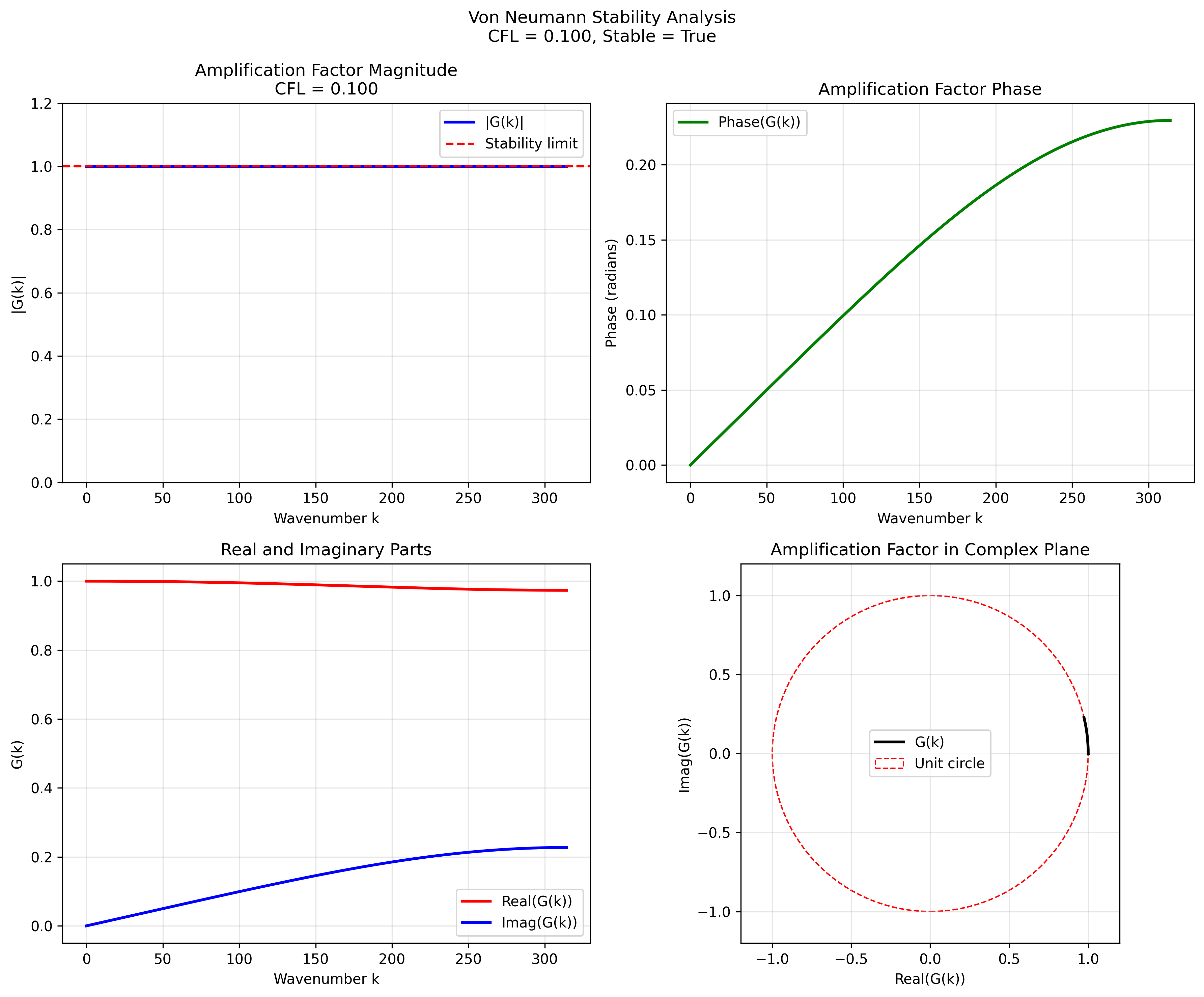CFL = 0.1 (stable regime)

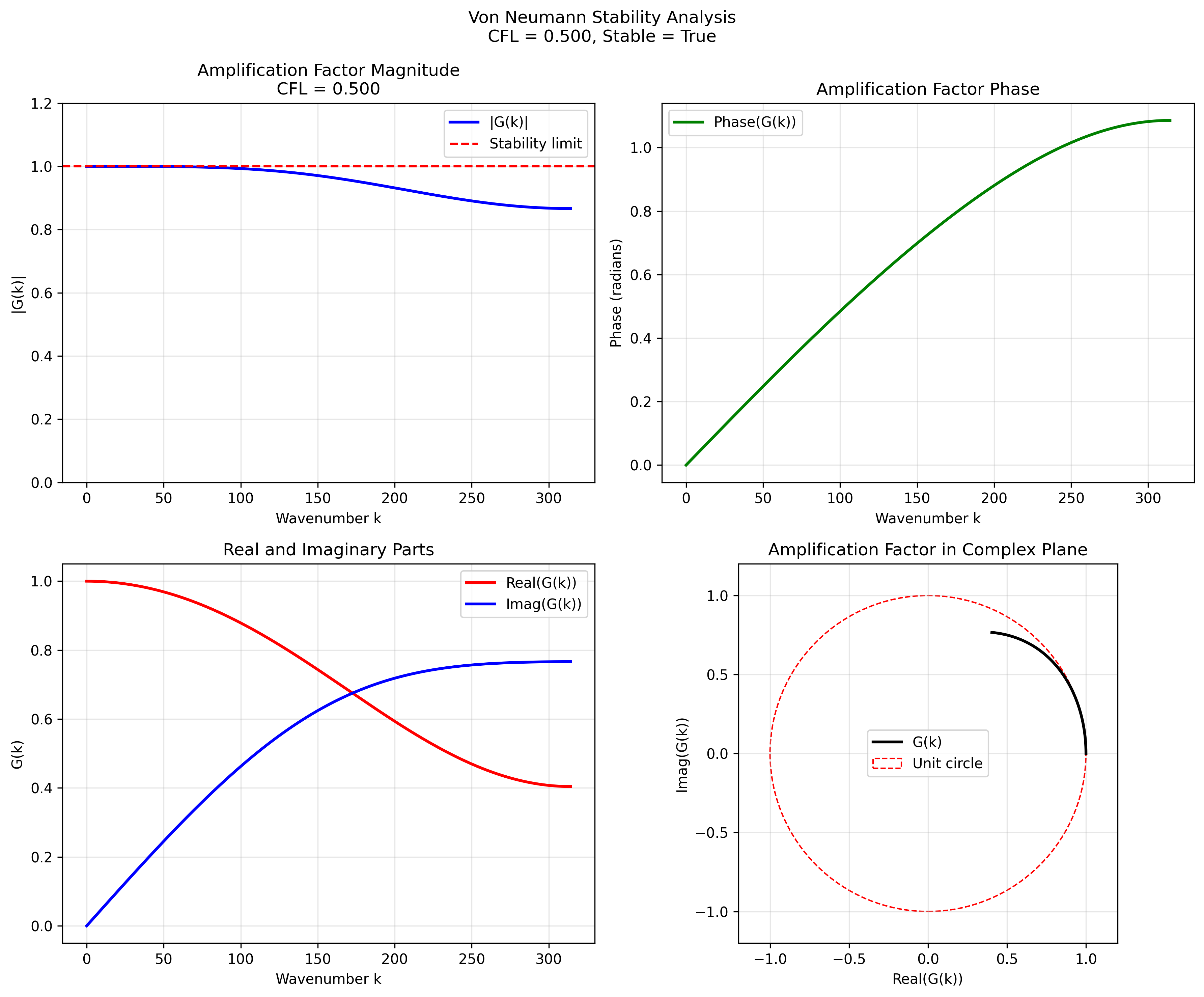CFL = 0.5 (critical CFL)

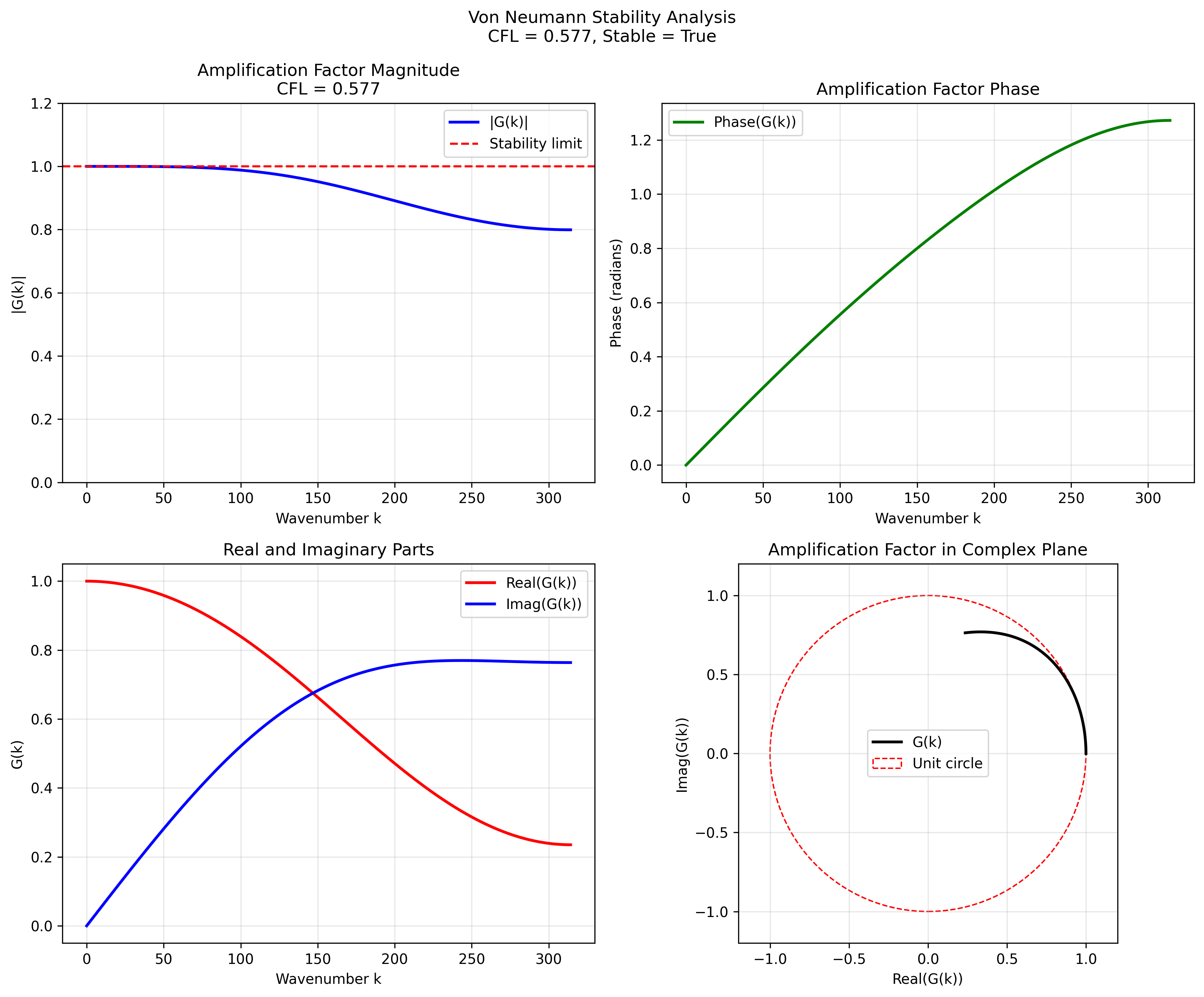CFL = 0.577 (theoretical 2nd-order 3D limit)

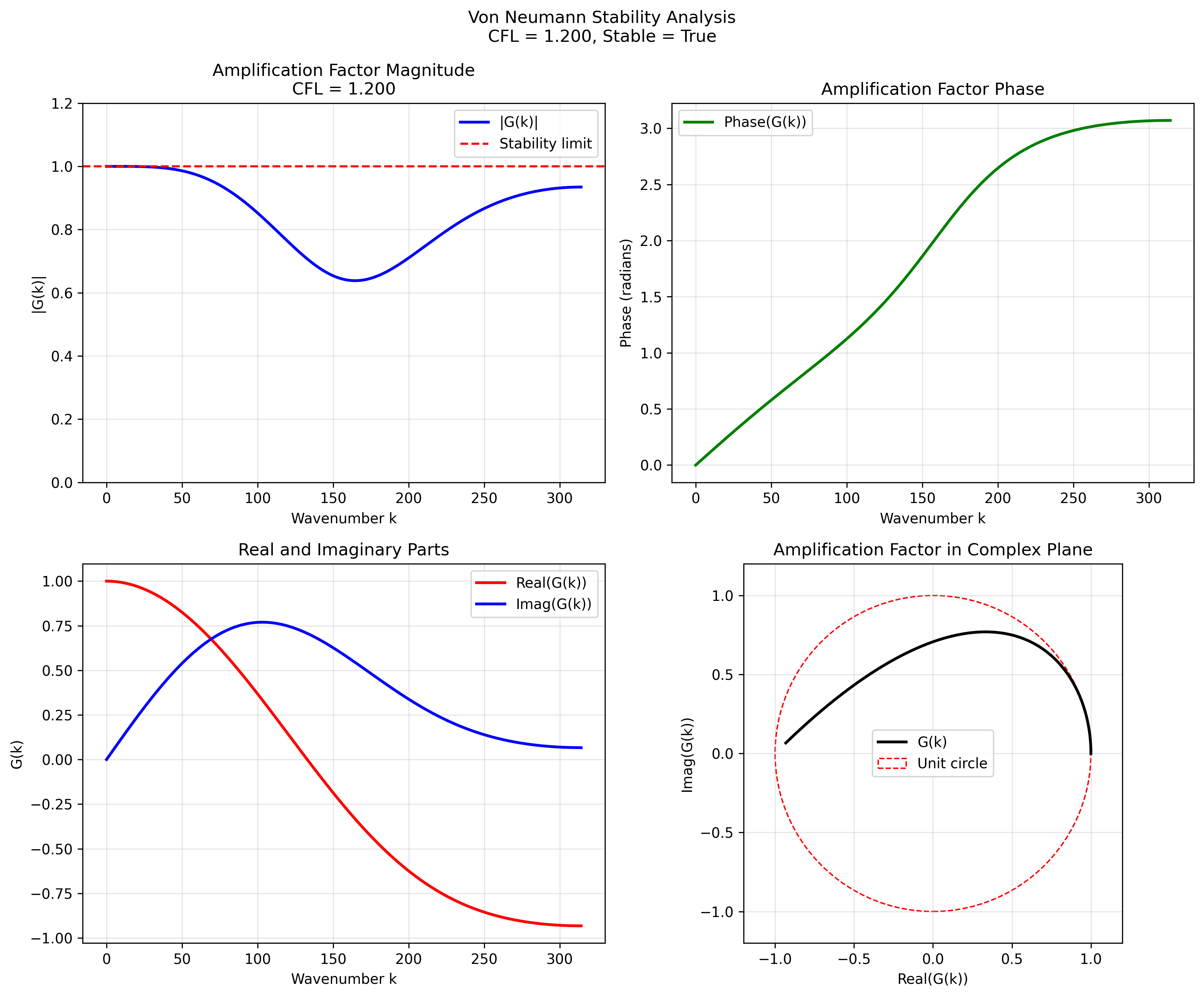CFL = 1.0 (unstable regime)

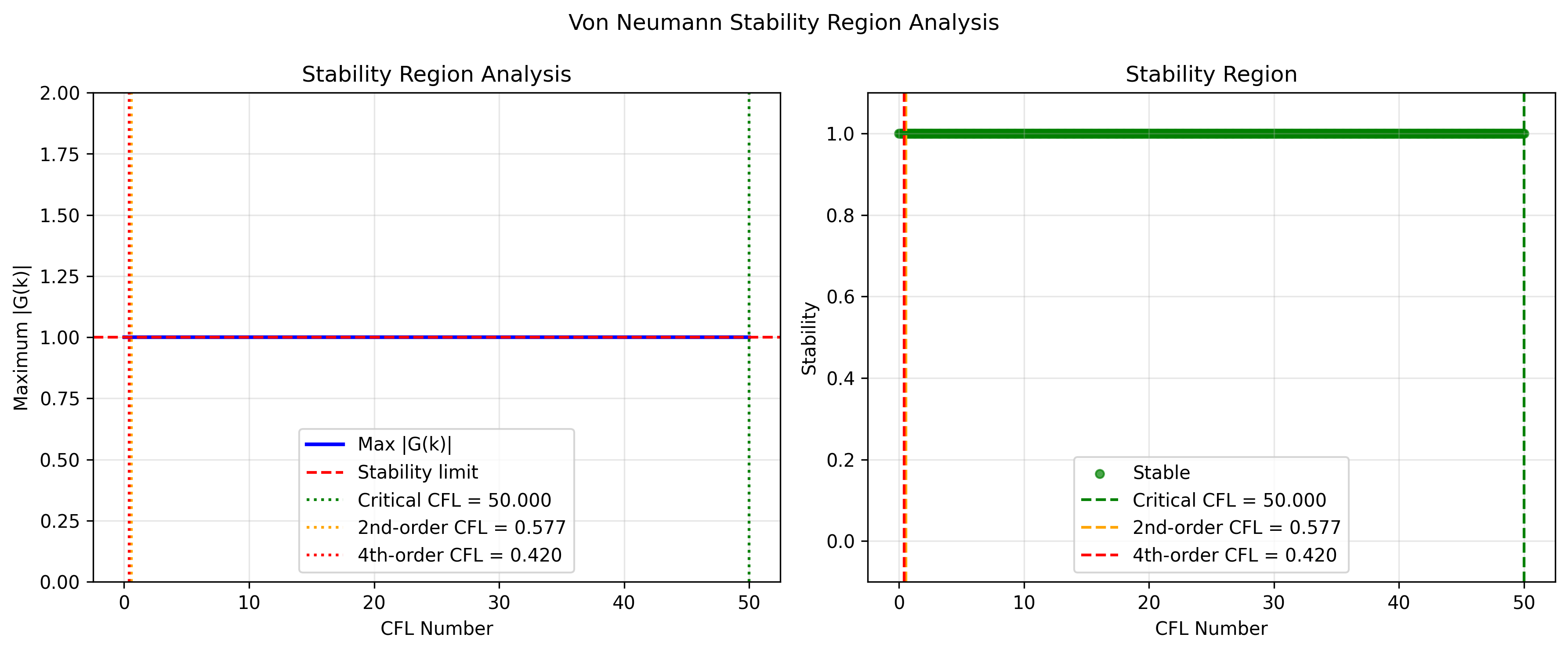Stability Region Analysis

Modified Wavenumber Analysis:

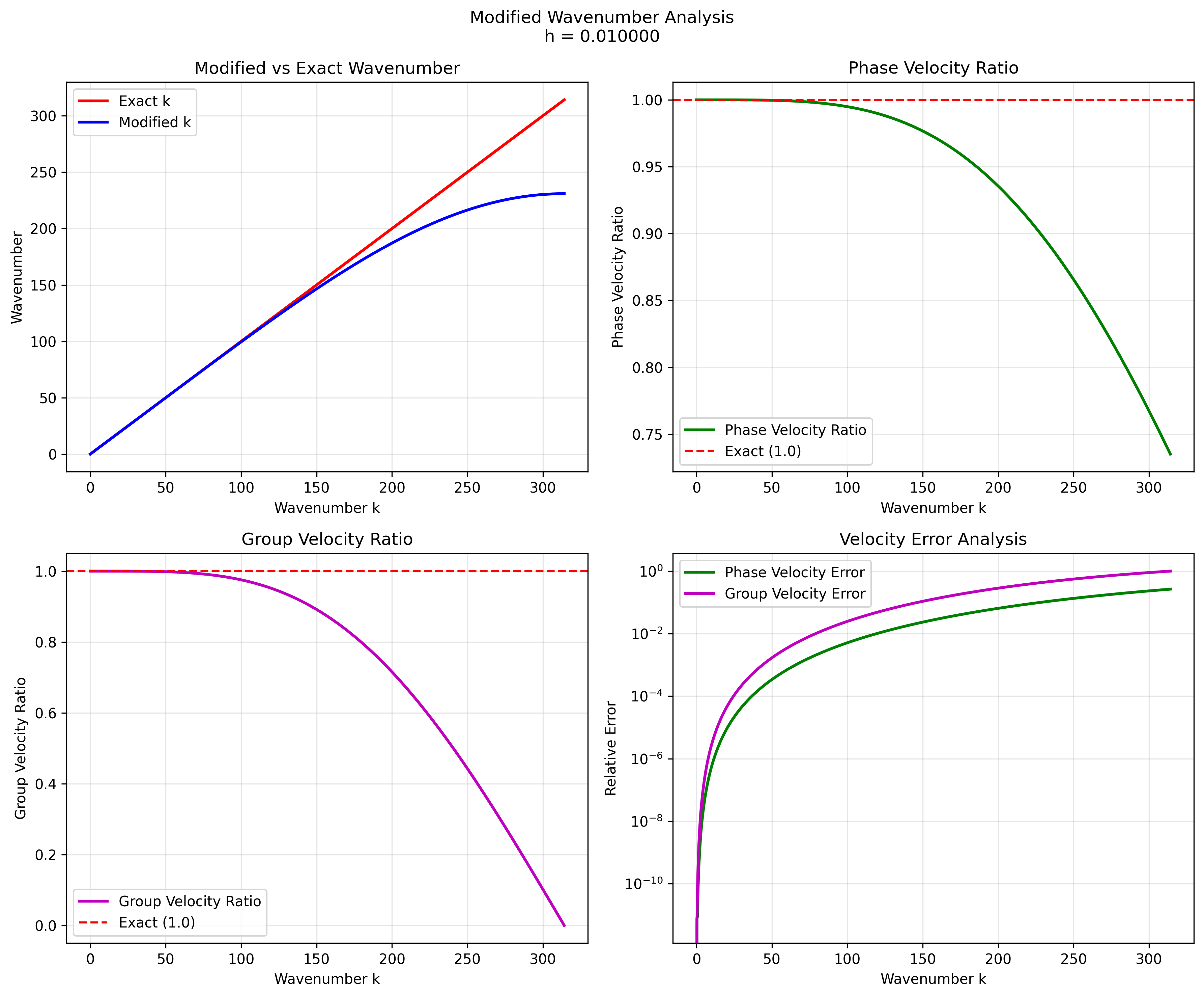Fine grid (h = 0.01)

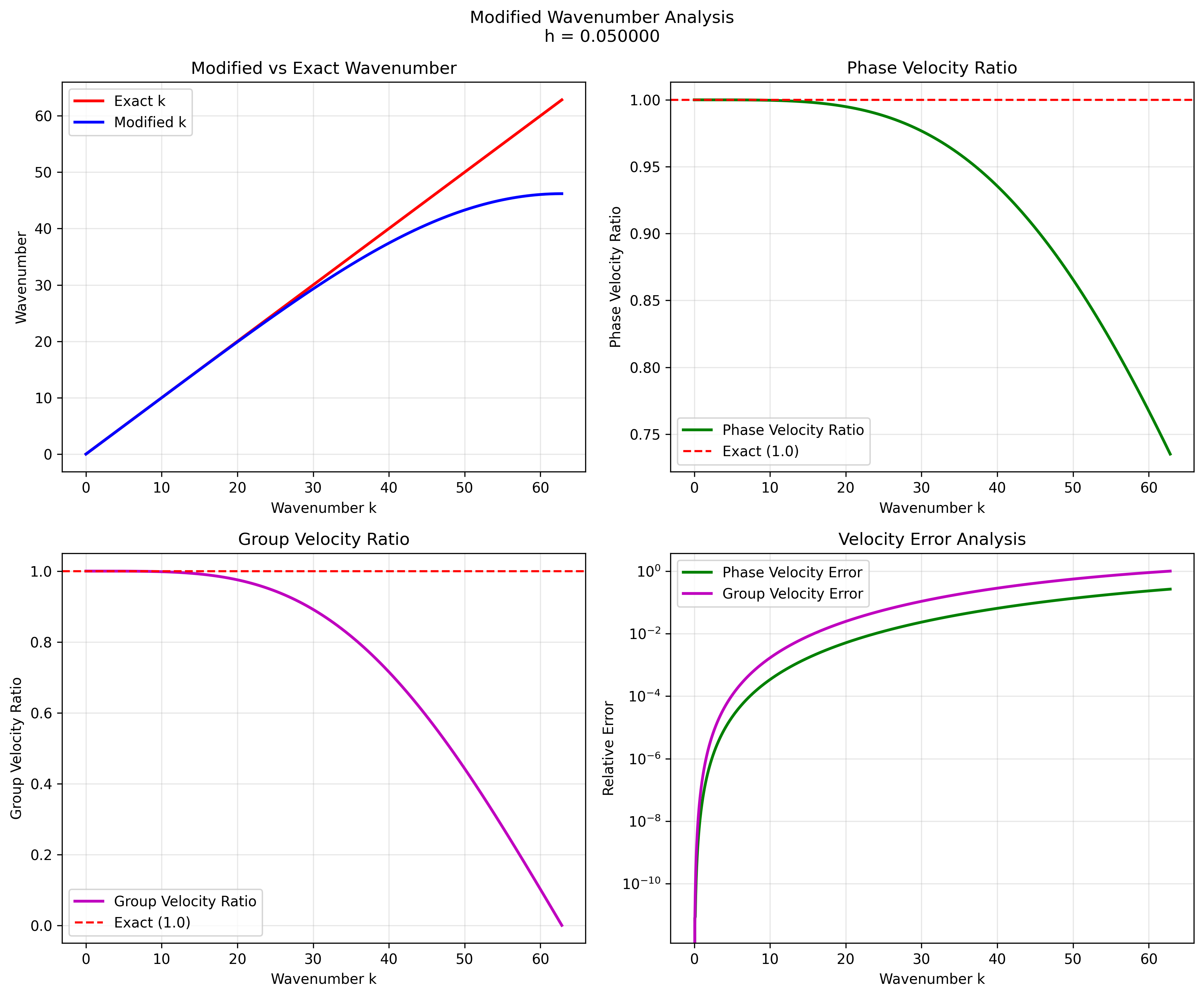Medium grid (h = 0.05)

Detailed Analysis Documentation

Note: Some initial theoretical analysis results were later found to be suspect and were corrected through real numerical testing. The final validated results are documented in this file and used in the correctness testing methodology.

Summary

The mathematical foundations provide:

1. Equation Identification: Confirms we’re solving the 3D wave equation with 4th-order spatial, 2nd-order temporal discretization
2. Stability Analysis: Establishes CFL < 0.5 constraint for all testing
3. Accuracy Characterization: Defines expected convergence rates and resolution requirements
4. Correctness Definition: Multi-level approach (parity, physical, stability, convergence)
5. Testing Methodology: Systematic validation at each level
6. Workflow Integration: Correctness-first approach ensures valid performance analysis
7. Analysis Tools: Python scripts for theoretical and numerical analysis

These foundations ensure that CUDA kernel optimization proceeds from a solid mathematical and numerical basis, with correctness validation at every step.