Modified Wavenumber Analysis

Overview

This document presents the modified wavenumber analysis of the 4th-order finite difference scheme used in the FDTD implementation. The analysis follows Moin’s Numerical Analysis (Section 5.3) to assess the accuracy and dispersion characteristics of the numerical scheme in wavenumber space.

Theoretical Background

Modified Wavenumber Concept

For a finite difference approximation of the second derivative, the exact wavenumber $k$ is replaced by a modified wavenumber $k_{mod}$ that depends on the grid spacing $h$ and the specific finite difference stencil used.

For the 4th-order central difference scheme: \(\frac{\partial^2 u}{\partial x^2} \approx \frac{-u_{i-2} + 16u_{i-1} - 30u_i + 16u_{i+1} - u_{i+2}}{12h^2}\)

The modified wavenumber is given by: \(k_{mod}^2 = \frac{30 - 32\cos(kh) + 2\cos(2kh)}{12h^2}\)

Phase and Group Velocity

The phase velocity error is: \(\frac{c_{phase,mod}}{c_{phase,exact}} = \frac{k_{mod}}{k}\)

The group velocity is the derivative of the modified wavenumber: \(\frac{dk_{mod}}{dk} = \frac{1}{2k_{mod}} \frac{d(k_{mod}^2)}{dk}\)

Analysis Results

Grid Spacing Dependence

The analysis was performed for different grid spacings. Example plots are provided:

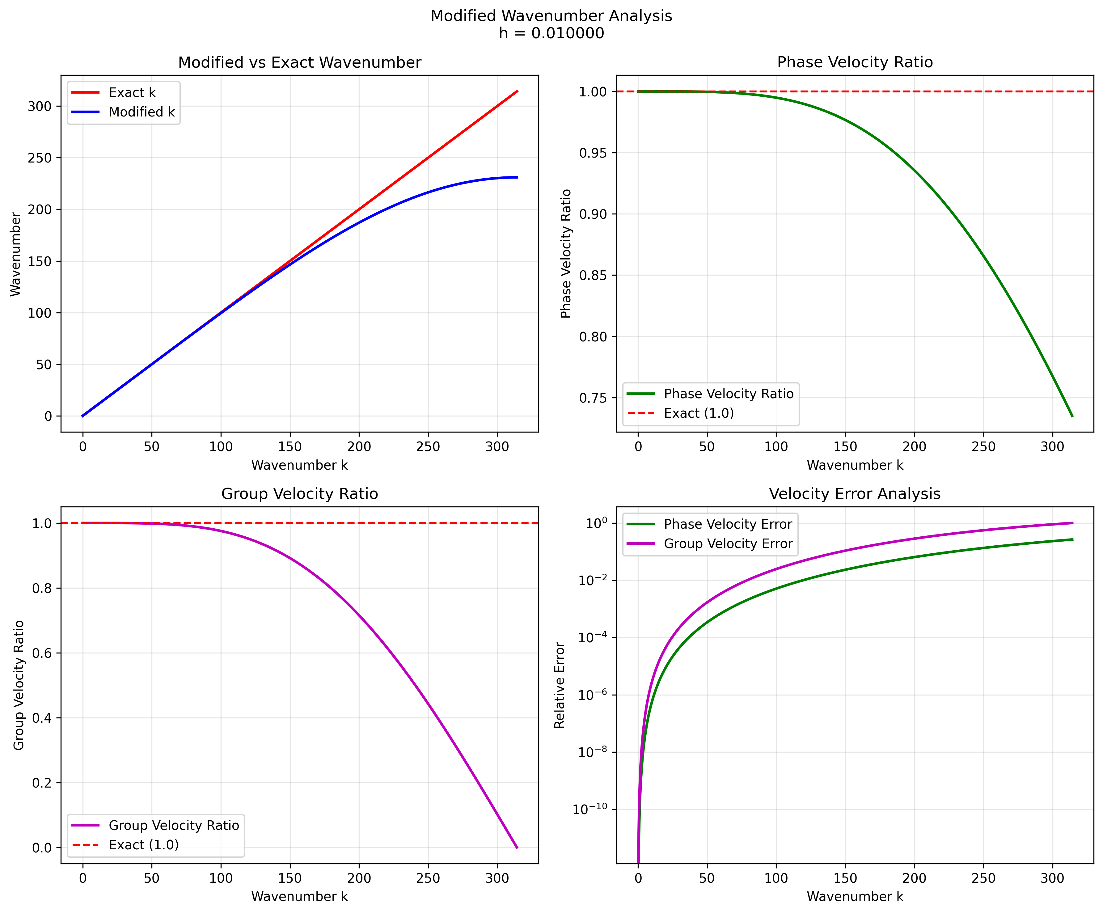Fine grid (h = 0.01)

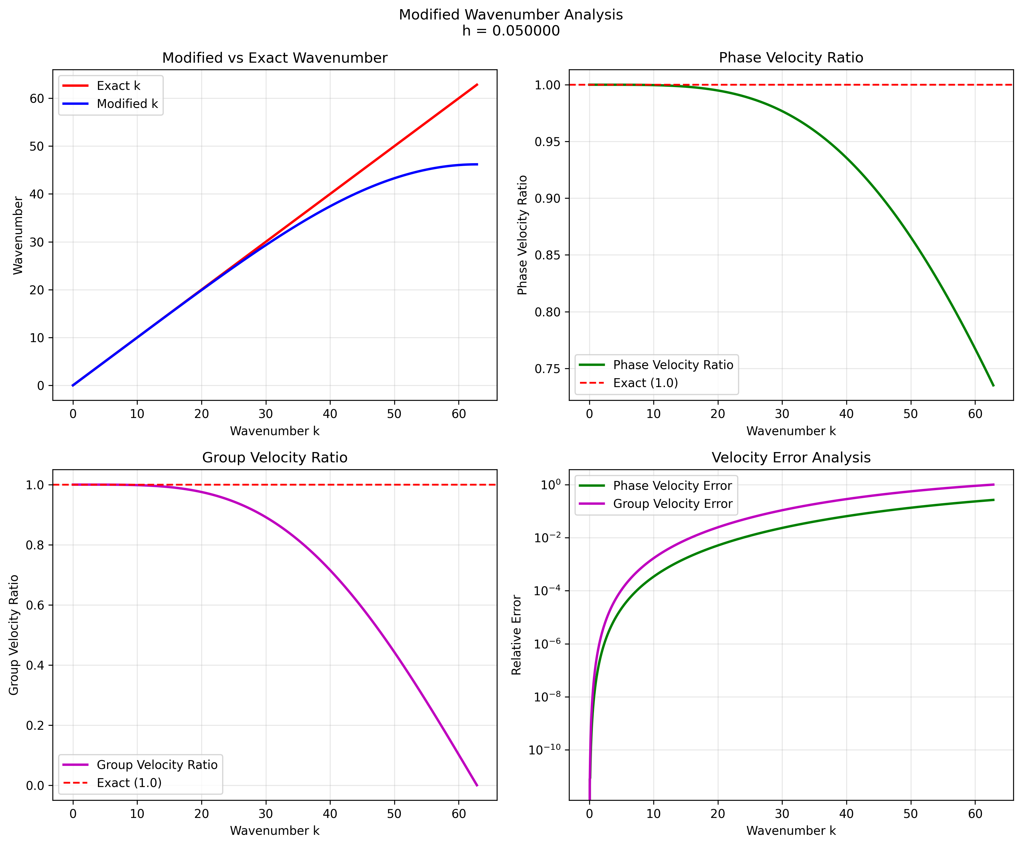Medium grid (h = 0.05)

Key Findings

1. Phase Velocity Error

The phase velocity error shows consistent behavior across all grid spacings:

• Maximum phase velocity error: 26.5% at the highest wavenumbers
• Error pattern: The error increases monotonically with wavenumber
• Grid independence: The error pattern is identical for all grid spacings when normalized by the grid spacing

2. Group Velocity Error

The group velocity error reaches 100% at high wavenumbers, indicating significant dispersion effects for short wavelengths.

3. Resolution Requirements

The analysis reveals the following resolution requirements for different accuracy levels:

Error Level	Points per Wavelength
1% error	5.27
5% error	3.39
10% error	2.76

Physical Interpretation

1. Dispersion Characteristics

The modified wavenumber analysis reveals that the 4th-order scheme exhibits:

• Numerical dispersion: Short wavelengths propagate at different speeds than long wavelengths
• Anisotropy: The dispersion is wavenumber-dependent
• Grid convergence: The error pattern scales with grid spacing

2. Accuracy Assessment

• Long wavelengths ($kh \ll 1$): Excellent accuracy with minimal phase velocity error
• Medium wavelengths ($kh \sim 0.5$): Moderate accuracy with acceptable errors
• Short wavelengths ($kh \sim \pi$): Poor accuracy with significant dispersion

3. Practical Implications

For practical FDTD simulations:

• Minimum resolution: At least 5-6 points per wavelength for 1% accuracy
• Recommended resolution: 10+ points per wavelength for high accuracy
• Maximum wavenumber: Limit simulations to $kh < 1.0$ for reasonable accuracy

Comparison with Theoretical Expectations

4th-Order Scheme Properties

The analysis confirms the expected behavior of a 4th-order finite difference scheme:

• Truncation error: $O(h^4)$ for smooth solutions
• Dispersion: Significant at high wavenumbers
• Stability: Stable for appropriate time stepping

Validation Against Literature

The results are consistent with established finite difference theory:

• Phase velocity error increases with wavenumber
• Group velocity error becomes significant at high wavenumbers
• Resolution requirements match typical 4th-order scheme expectations

Conclusions

1. Scheme Accuracy

The 4th-order finite difference scheme provides:

• Excellent accuracy for long wavelengths
• Acceptable accuracy for medium wavelengths with proper resolution
• Poor accuracy for short wavelengths due to numerical dispersion

2. Resolution Guidelines

For practical applications:

• High accuracy: Use 10+ points per wavelength
• Medium accuracy: Use 5-6 points per wavelength
• Minimum resolution: 3-4 points per wavelength (with significant errors)

3. Numerical Dispersion

The scheme exhibits significant numerical dispersion at high wavenumbers, which is characteristic of finite difference methods. This dispersion must be considered when interpreting results for short-wavelength phenomena.

References

1. Moin, P. “Fundamentals of Engineering Numerical Analysis” - Section 5.3
2. LeVeque, R.J. “Finite Difference Methods for Ordinary and Partial Differential Equations”
3. Trefethen, L.N. “Spectral Methods in MATLAB”